Modal analysis

---

---

General formulation of the problem

---

The goal of modal analysis is to determine the natural mode shapes and frequencies of an object or structure during free vibration. Let us again consider the problem of elastodynamics (neglecting the volumetric force)

\begin{equation} \rho \ddot{\mathbf{u}} = \operatorname{div} \sigma, \quad \text{in $\Omega$} \end{equation}

where \(\boldsymbol{\sigma}\) denotes the stress tensor which is, for an isotropic material, given by

\begin{equation} \boldsymbol{\sigma}=\lambda\mathrm{tr}(\boldsymbol{\varepsilon})\mathbf{I} + 2\mu\boldsymbol{\varepsilon}, \end{equation}

where the strain tensor \(\boldsymbol{\varepsilon}\) takes the form

\begin{equation} \boldsymbol{\varepsilon}=\frac{1}{2}\left(\nabla\mathbf{u}+ \left( \nabla\mathbf{u} \right)^{\top} \right), \end{equation}

while \(\lambda, \mu\) are Lame’s constants which can be expressed in terms of the Young’s modulus \(E\) and Poisson’s ratio \(\nu\) as

\begin{equation} \lambda = \frac{E \nu}{(1 + \nu) (1 - 2 \nu)}, \qquad \mu = \frac{E}{2(1 + \nu)}. \end{equation}

Testing the governing equation by \(\delta\mathbf{u}\), integrating over the spatial domain \(\Omega\), and integrating by parts yields the weak formulation of our problem. That is, find \(\mathbf{u}\) such that

\begin{equation} \int_\Omega \boldsymbol{\sigma}:\delta\boldsymbol{\varepsilon} \,\mathrm{dV} + \int_\Omega \rho\ddot{\mathbf{u}}\cdot\delta\mathbf{u} \,\mathrm{dV} = 0, \quad \forall \delta\mathbf{u}, \end{equation}

where \(\delta\boldsymbol{\varepsilon}\) is the symmetric gradient of \(\delta\mathbf{u}\). To perform the modal analysis we first assume that the displacement field takes the following form (referred to as normal mode)

\begin{equation} \mathbf{u}(\mathbf{x}, t)=\mathbf{u}_A(\mathbf{x})\mathrm{e}^{\mathrm{i}\omega t}, \end{equation}

where \(\mathbf{u}_A\) denotes the amplitude of the oscillating mode and \(\omega\) denotes the frequency of the mode. As a consequence we get

\begin{equation} \ddot{\mathbf{u}}(\mathbf{x}, t) = -\omega^2\mathbf{u}_A(\mathbf{x})\mathrm{e}^{\mathrm{i}\omega t} = -\omega^2 \mathbf{u}(\mathbf{x}, t), \end{equation}

and the weak formulation thus reduces to the following problem

\begin{equation} \int_\Omega \boldsymbol{\sigma}:\delta\boldsymbol{\varepsilon} \, \mathrm{dV} - \omega^2 \int_\Omega \rho\mathbf{u}\cdot\delta\mathbf{u} \,\mathrm{dV} = 0, \quad \forall \delta\mathbf{u}. \end{equation}

This formulation represents an eigenvalue problem which cannot be solved by the default FEniCS solver. The problem needs to be reformulated into an algebraic (generalized) eigenvalue problem

\begin{equation} \mathbf{A}\mathbf{u} - \omega^2\mathbf{M}\mathbf{u} = \mathbf{0}, \end{equation}

where \(\mathbf{A}\), \(\mathbf{M}\) are matrices assembled from the governing equations. This reformulation can be done easily in FEniCS, as well as solving the algebraic problem itself.

Implementation

---

As our model example we consider a 3D plate whose mesh is generated by the BoxMesh function. We do not prescribe any Dirichlet boundary condition. Otherwise, the first blocks of code are practically the same as in the previous examples so we do not comment them further.

import fenics as fe
import matplotlib.pyplot as plt


# --------------------
# Functions and classes
# --------------------
# Strain function
def epsilon(u):
    return 0.5*(fe.nabla_grad(u) + fe.nabla_grad(u).T)

# Stress function
def sigma(u):
    return lmbda*fe.div(u)*fe.Identity(3) + 2*mu*epsilon(u)

# --------------------
# Parameters
# --------------------
# Young modulus, poisson number and density
E, nu = 70.0E9, 0.23
rho = 2500.0

# Lame's constants
mu = E/2./(1+nu)
lmbda = E*nu/(1+nu)/(1-2*nu)

l_x, l_y, l_z = 1.0, 1.0, 0.01  # Domain dimensions
n_x, n_y, n_z = 20, 20, 2  # Number of elements

# --------------------
# Geometry
# --------------------
mesh = fe.BoxMesh(fe.Point(0.0, 0.0, 0.0), fe.Point(l_x, l_y, l_z), n_x, n_y, n_z)

# --------------------
# Function spaces
# --------------------
V = fe.VectorFunctionSpace(mesh, "CG", 2)
u_tr = fe.TrialFunction(V)
u_test = fe.TestFunction(V)

Next, we define the weak formulation of our problem.

# --------------------
# Forms & matrices
# --------------------
a_form = fe.inner(sigma(u_tr), epsilon(u_test))*fe.dx
m_form = rho*fe.inner(u_tr, u_test)*fe.dx

Now, we create two PETScMatrix() objects that will hold the matrices assembled from the weak formulation. (PETSc is a widely used library for sparse matrix computations.) By calling fe.assemble(), FEniCS performs integration and localization and outputs the result as a matrix or a vector. The last two lines assemble the standard stiffness matrix A and mass matrix M.

A = fe.PETScMatrix()
M = fe.PETScMatrix()
A = fe.assemble(a_form, tensor=A)
M = fe.assemble(m_form, tensor=M)

If we want apply Dirichlet boundary condition on matrices A and M, we call .zero method of DirichletBC object. For example for bc object as bc.zero(A) and bc.zero(M).

The first step for solving the algebraic eigenvalue problem lies in creating an instance of the SLEPcEigenSolver constructor with two arguments: the stiffness matrix A and the mass matrix M.

# --------------------
# Eigen-solver
# --------------------
fe.PETScOptions.set("eps_view")
eigensolver = fe.SLEPcEigenSolver(A, M)

Various parameters of the instance eigensolver are then set to control the solver.

eigensolver.parameters["problem_type"] = "gen_hermitian"
eigensolver.parameters["spectrum"] = "smallest real"
eigensolver.parameters["spectral_transform"] = "shift-and-invert"
eigensolver.parameters["spectral_shift"] = 100.0

The possible choices for these parameters are summarized below.

“problem_type”	Description
“hermitian”	Hermitian
“non_hermitian”	Non-Hermitian
“gen_hermitian”	Generalized Hermitian
“gen_non_hermitian ”	Generalized Non-Hermitian
“pos_gen_non_herm itian”	Generalized Non-Hermitian with positive semidefinite M

“spectrum”	Description
“largest magnitude”	eigenvalues with largest magnitude
“smallest magnitude”	eigenvalues with smallest magnitude
“largest real”	eigenvalues with largest double part
“smallest real”	eigenvalues with smallest double part
“largest imaginary”	eigenvalues with largest imaginary part
“smallest imaginary”	eigenvalues with smallest imaginary part
“target magnitude”	eigenvalues closest to target in magnitude (versions >= 3.1)
“target real”	eigenvalues closest to target in real part (versions >= 3.1)
“target imaginary”	eigenvalues closest to target in imaginary part (versions >= 3.1)

“spectral_transform”	Description
“shift-and-invert”	A shift-and-invert transform
” “	No spectral transform

More information about the solver’s parameters can be found in the Dolfin documentation.

The eigenvalue problem is then solved by the solve() method which takes one parameter: the number of eigenvalues to be calculated.

N_eig = 12   # number of eigenvalues
eigensolver.solve(N_eig)

The solution is contained in the eigensolver object. We shall extract it and save it to an .xdmf file. For this purpose we create an instance of the XDMFFile() constructor and set some of its parameters. If true, the parameter flush_output allows one to inspect the results while the process is still running. Similarly, if true, the parameter functions_share_mesh optimizes the saving process by considering that all functions have the same mesh.

# --------------------
# Post-process
# --------------------
# Set up file for exporting results
file_results = fe.XDMFFile("MA.xdmf")
file_results.parameters["flush_output"] = True
file_results.parameters["functions_share_mesh"] = True

Finally, for each eigenvalue we calculate the corresponding eigenfrequency and save the corresponding eigenvector as a FeniCS Function.

# Eigenfrequencies
for i in range(0, N_eig):
    # Get i-th eigenvalue and eigenvector
    # r - real part of eigenvalue
    # c - imaginary part of eigenvalue
    # rx - real part of eigenvector
    # cx - imaginary part of eigenvector
    r, c, rx, cx = eigensolver.get_eigenpair(i)

    # Calculation of eigenfrequency from real part of eigenvalue
    freq_3D = fe.sqrt(r)/2/fe.pi
    print("Eigenfrequency: {0:8.5f} [Hz]".format(freq_3D))

    # Initialize function and assign eigenvector
    eigenmode = fe.Function(V, name="Eigenvector " + str(i))
    eigenmode.vector()[:] = rx

    # Write i-th eigenfunction to xdmf file
    file_results.write(eigenmode, i)

Eigenfrequency:  0.00814 [Hz]
Eigenfrequency:  0.00835 [Hz]
Eigenfrequency:  0.00857 [Hz]
Eigenfrequency:  0.01140 [Hz]
Eigenfrequency:  0.01184 [Hz]
Eigenfrequency:  0.01208 [Hz]
Eigenfrequency: 35.16121 [Hz]
Eigenfrequency: 50.83763 [Hz]
Eigenfrequency: 59.78057 [Hz]
Eigenfrequency: 89.80385 [Hz]
Eigenfrequency: 90.36883 [Hz]
Eigenfrequency: 153.76596 [Hz]

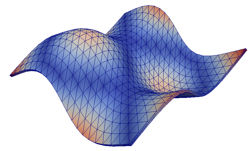
Here are two examples of the computed eigenmodes which are visualized using the external tool ParaView.

First eigenmode.	Fifth eigenmode.

Complete code

---

import fenics as fe
import matplotlib.pyplot as plt


# --------------------
# Functions and classes
# --------------------
# Strain function
def epsilon(u):
    return 0.5*(fe.nabla_grad(u) + fe.nabla_grad(u).T)

# Stress function
def sigma(u):
    return lmbda*fe.div(u)*fe.Identity(3) + 2*mu*epsilon(u)

# --------------------
# Parameters
# --------------------
# Young modulus, poisson number and density
E, nu = 70.0E9, 0.23
rho = 2500.0

# Lame's constants
mu = E/2./(1+nu)
lmbda = E*nu/(1+nu)/(1-2*nu)

l_x, l_y, l_z = 1.0, 1.0, 0.01  # Domain dimensions
n_x, n_y, n_z = 20, 20, 2  # Number of elements

# --------------------
# Geometry
# --------------------
mesh = fe.BoxMesh(fe.Point(0.0, 0.0, 0.0), fe.Point(l_x, l_y, l_z), n_x, n_y, n_z)

# --------------------
# Function spaces
# --------------------
V = fe.VectorFunctionSpace(mesh, "CG", 2)
u_tr = fe.TrialFunction(V)
u_test = fe.TestFunction(V)

# --------------------
# Forms & matrices
# --------------------
a_form = fe.inner(sigma(u_tr), epsilon(u_test))*fe.dx
m_form = rho*fe.inner(u_tr, u_test)*fe.dx

A = fe.PETScMatrix()
M = fe.PETScMatrix()
A = fe.assemble(a_form, tensor=A)
M = fe.assemble(m_form, tensor=M)

# --------------------
# Eigen-solver
# --------------------
eigensolver = fe.SLEPcEigenSolver(A, M)
eigensolver.parameters['problem_type'] = 'gen_hermitian'
eigensolver.parameters["spectrum"] = "smallest real"
eigensolver.parameters['spectral_transform'] = 'shift-and-invert'
eigensolver.parameters['spectral_shift'] = 100.0

N_eig = 12   # number of eigenvalues
eigensolver.solve(N_eig)

# --------------------
# Post-process
# --------------------
# Set up file for exporting results
file_results = fe.XDMFFile("MA.xdmf")
file_results.parameters["flush_output"] = True
file_results.parameters["functions_share_mesh"] = True

# Eigenfrequencies
for i in range(0, N_eig):
    # Get i-th eigenvalue and eigenvector
    # r - real part of eigenvalue
    # c - imaginary part of eigenvalue
    # rx - real part of eigenvector
    # cx - imaginary part of eigenvector
    r, c, rx, cx = eigensolver.get_eigenpair(i)

    # Calculation of eigenfrequency from real part of eigenvalue
    freq_3D = fe.sqrt(r)/2/fe.pi
    print("Eigenfrequency: {0:8.5f} [Hz]".format(freq_3D))

    # Initialize function and assign eigenvector
    eigenmode = fe.Function(V, name="Eigenvector " + str(i))
    eigenmode.vector()[:] = rx

    # Write i-th eigenfunction to xdmf file
    file_results.write(eigenmode, i)

Eigenfrequency:  0.00814 [Hz]
Eigenfrequency:  0.00835 [Hz]
Eigenfrequency:  0.00857 [Hz]
Eigenfrequency:  0.01140 [Hz]
Eigenfrequency:  0.01184 [Hz]
Eigenfrequency:  0.01208 [Hz]
Eigenfrequency: 35.16121 [Hz]
Eigenfrequency: 50.83763 [Hz]
Eigenfrequency: 59.78057 [Hz]
Eigenfrequency: 89.80385 [Hz]
Eigenfrequency: 90.36883 [Hz]
Eigenfrequency: 153.76596 [Hz]