2D Hyper-elasticity

---

---

General formulation of the problem

---

Let us consider a deformation

\begin{equation} \mathbf{y}(\mathbf{X}):=\mathbf{X} + \mathbf{u}(\mathbf{X}), \end{equation}

as on the picture (REF) above (we denote \(\chi\) by \(\mathbf{y}\)) and let us denote by

\begin{equation} \mathbf{F}(\mathbf{X}):=\mathrm{Grad}\,\mathbf{y}(\mathbf{X}), \end{equation}

its gradient. The lenght, surface area and volume are then transformed by

\begin{align*} \mathrm{d}l &= \mathbf{F}\,\mathrm{d}L, \\ \mathrm{d}s &= (\mathrm{det}\,\mathbf{F})\mathbf{F}^{-\top}\mathrm{d}S, \\ \mathrm{d}v &= \mathrm{det}\mathbf{F}\,\mathrm{d}V, \end{align*}

respectively. It follows then that the unit normal \(\mathbf{N}\) in the reference configuration and the corresponding unit normal in the deformed configuration are related by

\begin{equation} \mathbf{n} = \frac{(\mathrm{det}\,\mathbf{F})\mathbf{F}^{-\top}\mathbf{N}} {|(\mathrm{det}\,\mathbf{F})\mathbf{F}^{-\top}\mathbf{N}|}. \end{equation}

For Lagrangian description it is more suitable to use the 1st Piola-Kirchhoff stress tensor \(\mathbf{P}\), which assings to a normal \(\mathbf{N}\) the corresponding traction in the deformed configuration. Its relation to the Cauchy stress tensor \({\boldsymbol \sigma}\) is

\begin{equation} \mathbf{P} = (\mathrm{det}\,\mathbf{F})\,{\boldsymbol \sigma}\,\mathbf{F}^{-\top}, \end{equation}

For rewriting the problem fully in the Lagrangian coordinates we will also transform the body and surface forces

\begin{align*} \mathbf{B} &= (\mathrm{det}\,\mathbf{F})\mathbf{b}, \\ \mathbf{G} &= |(\mathrm{det}\,\mathbf{F})\mathbf{F}^{-\top}\mathbf{N}|\,\mathbf{g}. \end{align*}

Using the Piola identity

\begin{equation} \mathrm{Div}\left[(\mathrm{det}\,\mathbf{F})\mathbf{F}^{-\top} \right] = \mathbf{0}, \end{equation}

we obtain that

\begin{equation} \mathrm{div}{\boldsymbol \sigma} = \mathrm{det}\mathbf{F}\,\mathrm{Div}\,\mathbf{P}. \end{equation}

Having all these formulas at hand, the original problem

\begin{align*} && \mathrm{div}\boldsymbol{\sigma} + \mathbf{b} &= \mathbf{0} && \text{in}\ \mathbf{y}(\Omega), \\ && \boldsymbol{\sigma} \cdot \mathbf{n} &= \mathbf{g}, && \text{on}\ \mathbf{y}(\Gamma_N), \\ && \mathbf{u} &= \bar{\mathbf{u}}, && \text{on}\ \mathbf{y}(\Gamma_D), \end{align*}

can be now easily rewritten in Lagrangian coordinates

\begin{align*} && \mathrm{Div}\,\mathbf{P} + \mathbf{B} &= \mathbf{0} && \text{in}\ \Omega, \\ && \mathbf{P}\cdot\mathbf{N} &= \mathbf{G}, && \text{on}\ \Gamma_N, \\ && \mathbf{u} &= \bar{\mathbf{u}}, && \text{on}\ \Gamma_D, \end{align*}

Purely formally, the problem above is nothing but the Euler-Lagrange equations of the energy functional

\begin{equation} I(\mathbf{u}) = \int_\Omega W(\mathbf{F}) \, \mathrm{d} V -\int_\Omega \mathbf{B} \cdot \mathbf{u} \, \mathrm{d} V -\int_{\partial \Omega} \mathbf{G} \cdot \mathbf{u} \, \mathrm{d} S \end{equation}

minimized over the displacements satisfying the dirichlet boundary condition. The 1st Piola-Kirchhoff stress tensor is then given by the stored energy density \(W\) by

\begin{align*} \mathbf{P} = \frac{\partial W}{\partial \mathbf{F}}. \end{align*}

We will profit form this in the sequel, since it is enough to prescribe the energy functional and the corresponding E-L equations are compouted in FEniCS automatically.

Choice of the stored energy function

Linear elasticity is well established. The symmetric gradient of displacement \(\boldsymbol{\varepsilon}\) is a good strain measure for small deformations and quadratic energy is the simplest choice working for broad range of materials. Its form is completely specified by its second derivative, the so-called tensor of elastic constants, whose experimental fitting is well known.

This is not true for large deformations, where the situation is much more complicated. There is no universal strain measure (by itself immaterial), nor a general ansatz for the stored energy function \(W\). Even though there are materials with same elastic moduli in the small deformations regime, their response differ significantly in large strain regime. Nevertheless, the tensor of elastic constants obtained from the quadratic envelope of \(W\) provides a good clue and even in some situations determines \(W\) completely.

Let us now mention a few examples of the most used stored energy densities of isotropic materials. Probably the simplest one is the St. Venant-Kirchhoff energy

\begin{align*} W(\mathbf{E}) &= \frac{\lambda}{2} (\mathrm{tr} \, \mathbf{E})^2 + \mu |\mathbf{E}|^2, && \mathbf{I} + 2 \mathbf{E} = \mathbf{F}^\top \mathbf{F}, \end{align*}

where the strain measure \(\boldsymbol{\varepsilon}\) was just replaced by the Green-St. Venant tensor \(E\). This energy depends explicitly on the known elastic constants and is therefore very popular among experimentalists. It lacks, however, other important properties. For example no existence theory is known for such an~energy, but here are others ‘more interesting from the engineering point of view’. It is known the material can be deformed in such a way that linear waves around this new configuration does not have a real speed of propagation. Hence we rather choose the Mooney-Rivlin energy

\begin{align*} W(\mathbf{F}) &= a |\mathbf{F}|^2 + b|J\mathbf{F}^{-\top}|^2 + cJ^2 - d\ln J + e, && J = \det \mathbf{F}. \end{align*}

The positive parameters (except of \(e\)) can be expressed in terms of the Lame constants \(\lambda\) and \(\mu\) in such a way that the Mooney-Rivlin energy approximates the St. Venant-Kirchhoff one for very small \(|\mathbf{E}|\); see e.g. [Ciarlet P.G. - Mathematical Elasticity (1988), Thm. 4.10-2]. For our purposes it will be sufficient to consider its simplified form, the so-called Neo-Hook energy

\begin{align*} W(\mathbf{F}) &= \frac{\mu}{2}( |\mathbf{F}|^2 - 3 - 2 \ln \det \mathbf{F} ), \end{align*}

where \(\mu\) is indeed the shear modulus (\(\lambda = 0\)), i.e. \(a=\frac{\mu}{2}\), \(b=c=0\), \(d = \mu\), and \(e = -\frac{3}{2}\). The last energy we mention here is the isotropic Hencky strain energy

\begin{align*} W(\mathbf{E}^H) &= \frac{\kappa}{2} (\mathrm{tr} \, \mathbf{E}^H)^2 + \mu |\mathbf{E}^H_0|^2 \end{align*}

where \(\kappa\) is the bulk modulus,

\begin{align*} \mathbf{E}^H = \frac{1}{2} \ln (\mathbf{F} \mathbf{F}^\top), \end{align*}

is the Hencky strain and

\begin{align*} \mathbf{E}^H_0 = \mathbf{E}^H - \frac{1}{3} (\text{tr}\, \mathbf{E}^H) \mathbf{I}, \end{align*}

is its deviatoric part. Note that

\begin{align*} && \text{tr } \mathbf{E}^H = \ln J, && \mathbf{E}^H_0 = \frac{1}{2} \ln \left( \frac{\mathbf{F} \mathbf{F}^\top}{J^{2/3}} \right). && \end{align*}

Although much more involved, this energy is in good agreement with experiments on a wide class of materials for principal stretches ranging between 0.7 and 1.3; see [Gurtin M. E., Fried E., Anand L. - The Mechanics and Thermodynamics of Continua (2010), p. 330] and references therein. However, a general existence theory for this energy is still out of reach.

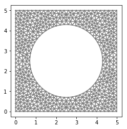
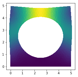
Computing deformation of an infinite cork tunnel

Now we will re-compute the 2D in-plane strain problem. Since cork is the material of this course (and because it makes our lifes easier by \(\lambda = \nu = 0\)), we choose

\begin{align*} \mu = \frac{E}{2(1 + \nu)} = \frac{E}{2} = 10 \text{ MPa}. \end{align*}

Implementation

---

import fenics as fe
import matplotlib.pyplot as plt
import numpy as np
import ufl

fe.set_log_level(13)

# --------------------
# Functions and classes
# --------------------
def bottom(x, on_boundary):
    return (on_boundary and fe.near(x[1], 0.0))


# Strain function
def epsilon(u):
    return 0.5*(fe.grad(u) + fe.grad(u).T)


# Stress function
def sigma(u):
    return lmbda*fe.div(u)*fe.Identity(2) + 2*mu*epsilon(u)


# --------------------
# Parameters
# --------------------
# Lame's constants
#lmbda = 1.25
#mu = 20

E = 20.0e6
mu = 0.5*E
rho_0 = 200.0

l_x, l_y = 5.0, 5.0  # Domain dimensions
n_x, n_y = 500, 500  # Number of elements

# Load
g_int = 1.0e5
b_int = -10.0

# --------------------
# Geometry
# --------------------
mesh = fe.Mesh("external_mesh.xml")

fe.plot(mesh)
plt.show()

# Definition of Neumann condition domain
boundaries = fe.MeshFunction("size_t", mesh, mesh.topology().dim() - 1)
boundaries.set_all(0)

top = fe.AutoSubDomain(lambda x: fe.near(x[1], 5.0))

top.mark(boundaries, 1)
ds = fe.ds(subdomain_data=boundaries)

# --------------------
# Function spaces
# --------------------
V = fe.VectorFunctionSpace(mesh, "CG", 1)
u_tr = fe.TrialFunction(V)
u_test = fe.TestFunction(V)
u = fe.Function(V)
g = fe.Constant((0.0, g_int))
b = fe.Constant((0.0, b_int))
N = fe.Constant((0.0, 1.0))

aa, bb, cc, dd, ee = 0.5*mu, 0.0, 0.0, mu, -1.5*mu

# --------------------
# Boundary conditions
# --------------------
bc = fe.DirichletBC(V, fe.Constant((0.0, 0.0)), bottom)

# --------------------
# Weak form
# --------------------
I = fe.Identity(2)
F = I + fe.grad(u)  # Deformation gradient
C = F.T*F  # Right Cauchy-Green tensor
J = fe.det(F)  # Determinant of deformation fradient

#psi = (aa*fe.tr(C) + bb*fe.tr(ufl.cofac(C)) + cc*J**2 - dd*fe.ln(J))*fe.dx - fe.dot(b, u)*fe.dx + fe.inner(f, u)*ds(1)
n = fe.dot(ufl.cofac(F), N)
surface_def = fe.sqrt(fe.inner(n, n))
psi = (aa*fe.inner(F, F) + ee - dd*fe.ln(J))*fe.dx - rho_0*J*fe.dot(b, u)*fe.dx + surface_def*fe.inner(g, u)*ds(1)

# --------------------
# Solver
# --------------------
Form = fe.derivative(psi, u, u_test)
Jac = fe.derivative(Form, u, u_tr)

problem = fe.NonlinearVariationalProblem(Form, u, bc, Jac)
solver = fe.NonlinearVariationalSolver(problem)
prm = solver.parameters
#prm["newton_solver"]["error_on_convergence"] = False
#fe.solve(Form == 0, u, bc, J=Jac, solver_parameters={"error_on_convergence": False})
solver.solve()

print(np.amax(u.vector()[:]))

# --------------------
# Post-process
# --------------------
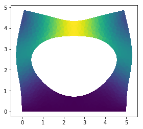
fe.plot(u, mode="displacement")
plt.show()

0.0923090480515

Comparison with linear elasticity

---

import fenics as fe
import matplotlib.pyplot as plt
import numpy as np
import ufl

fe.set_log_level(13)

# --------------------
# Functions and classes
# --------------------
def bottom(x, on_boundary):
    return (on_boundary and fe.near(x[1], 0.0))


# Strain function
def epsilon(u):
    return 0.5*(fe.grad(u) + fe.grad(u).T)


# Stress function
def sigma(u):
    return lmbda*fe.div(u)*fe.Identity(2) + 2*mu*epsilon(u)


def calc_linear():
    fe.solve(a == l, u_small, bc)
    return u_small((2.5, 5.0))[1]


def calc_nonlinear():
    Form = fe.derivative(psi, u_large, u_test)
    Jac = fe.derivative(Form, u_large, u_tr)

    problem = fe.NonlinearVariationalProblem(Form, u_large, bc, Jac)
    solver = fe.NonlinearVariationalSolver(problem)
    prm = solver.parameters
    prm["newton_solver"]["error_on_nonconvergence"] = False
    solver.solve()

    return u_large((2.5, 5.0))[1]


# --------------------
# Parameters
# --------------------
# Lame's constants
#lmbda = 1.25
#mu = 20

E = 20.0e6
mu = 0.5*E
rho_0 = 200.0

# Lame's constants
lmbda = 0.0

l_x, l_y = 5.0, 5.0  # Domain dimensions
n_x, n_y = 500, 500  # Number of elements

# Load
#g_int = fe.Expression("t", t=0, degree=0)
b_int = -10.0

# --------------------
# Geometry
# --------------------
mesh = fe.Mesh("external_mesh.xml")

fe.plot(mesh)
plt.show()

# Definition of Neumann condition domain
boundaries = fe.MeshFunction("size_t", mesh, mesh.topology().dim() - 1)
boundaries.set_all(0)

top = fe.AutoSubDomain(lambda x: fe.near(x[1], 5.0))

top.mark(boundaries, 1)
ds = fe.ds(subdomain_data=boundaries)

# --------------------
# Function spaces
# --------------------
V = fe.VectorFunctionSpace(mesh, "CG", 1)
u_tr = fe.TrialFunction(V)
u_test = fe.TestFunction(V)
u_small = fe.Function(V)
u_large = fe.Function(V)
g = fe.Expression((0.0, "t"), t=0, degree=0)
b = fe.Constant((0.0, b_int))
N = fe.Constant((0.0, 1.0))

aa, bb, cc, dd, ee = 0.5*mu, 0.0, 0.0, mu, -1.5*mu
pseudo_time = np.linspace(0.0, 3.5e5, 100)

# --------------------
# Boundary conditions
# --------------------
bc = fe.DirichletBC(V, fe.Constant((0.0, 0.0)), bottom)

# --------------------
# Weak form
# --------------------
I = fe.Identity(2)
F = I + fe.grad(u_large)  # Deformation gradient
C = F.T*F  # Right Cauchy-Green tensor
J = fe.det(F)  # Determinant of deformation fradient

#psi = (aa*fe.tr(C) + bb*fe.tr(ufl.cofac(C)) + cc*J**2 - dd*fe.ln(J))*fe.dx - fe.dot(b, u)*fe.dx + fe.inner(f, u)*ds(1)
n = fe.dot(ufl.cofac(F), N)
surface_def = fe.sqrt(fe.inner(n, n))
psi = (aa*fe.inner(F, F) + ee - dd*fe.ln(J))*fe.dx - rho_0*J*fe.dot(b, u_large)*fe.dx + surface_def*fe.inner(g, u_large)*ds(1)

a = fe.inner(sigma(u_tr), epsilon(u_test))*fe.dx
l = rho_0*fe.dot(b, u_test)*fe.dx - fe.inner(g, u_test)*ds(1)

# --------------------
# Time-loop
# --------------------
u_lin = []
u_nlin = []
for ti in pseudo_time:
    g.t = ti
    u_lin.append(calc_linear()*1000.0)
    u_nlin.append(calc_nonlinear()*1000.0)

# --------------------
# Post-process
# --------------------
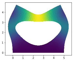
fe.plot(u_small, mode="displacement")
plt.show()
fe.plot(u_large, mode="displacement")
plt.show()
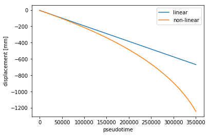
plt.plot(pseudo_time, u_lin, label="linear")
plt.plot(pseudo_time, u_nlin, label="non-linear")
plt.xlabel("pseudotime")
plt.ylabel("displacement [mm]")
plt.legend()
plt.show()